Crafting Your Own Stable Diffusion LoRA Using Free Cloud GPUs - Complete Guide 2025

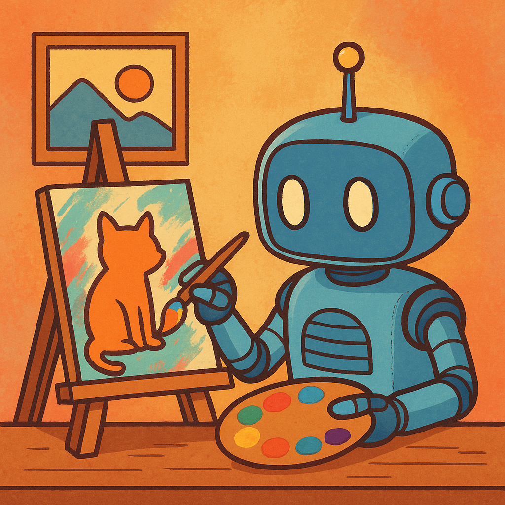
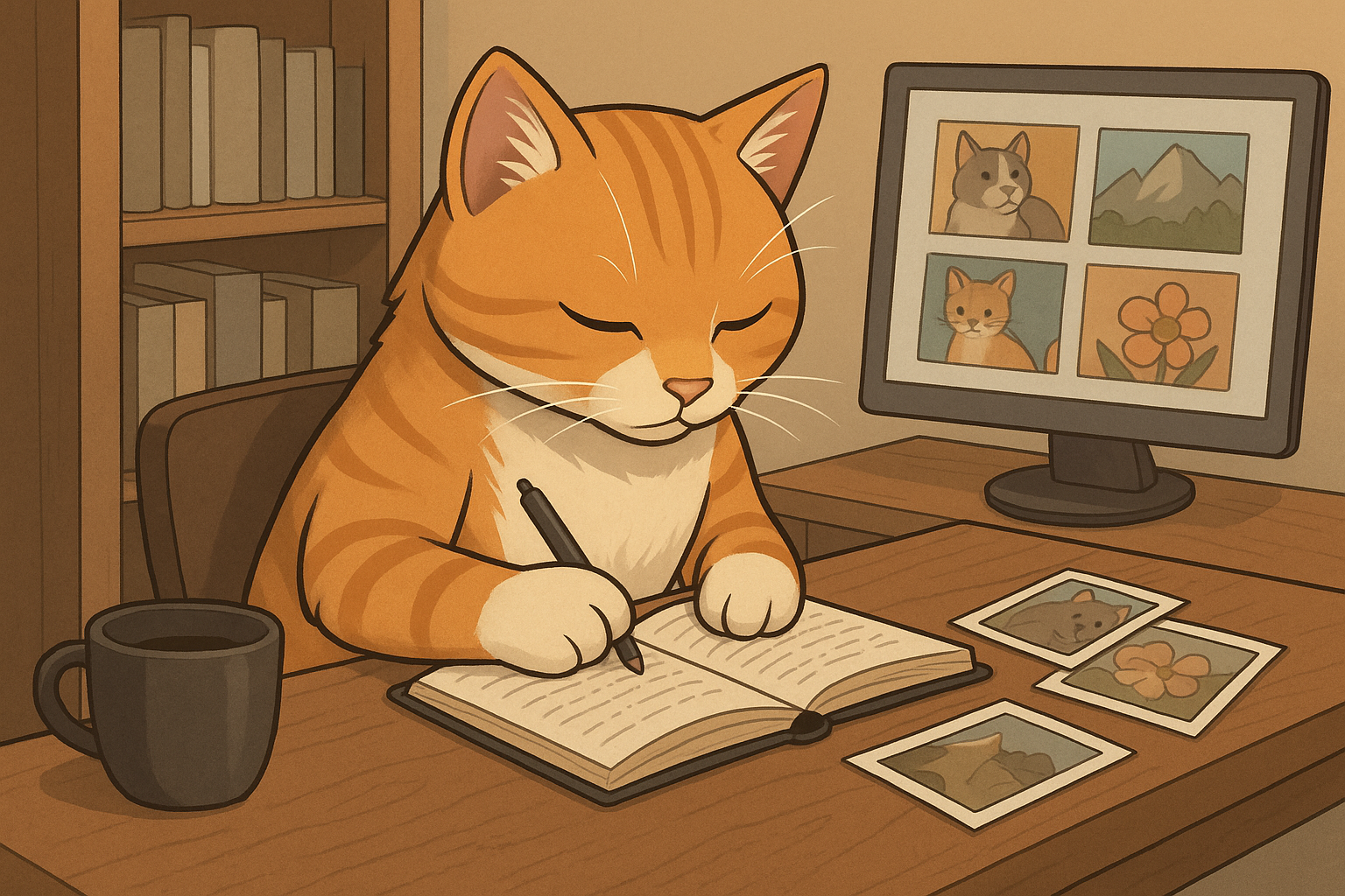
Welcome to the cloud‑powered edition of our Stable Diffusion tutorial! In this guide you'll learn how diffusion models work, why LoRA (Low‑Rank Adaptation) is a smart way to teach a model new tricks, and—most importantly—how to train a LoRA without owning a beefy GPU.

We'll use Kaggle's free GPU notebooks as our primary platform, though you can apply the same workflow to other free cloud services like Google Colab or Lightning.AI. Kaggle offers Tesla P100 GPUs with about 13 GB of VRAM and limits sessions to nine hours with a total of 30 GPU hours per week. If your PC lacks the VRAM needed for SDXL, using a cloud GPU service such as Colab or RunPod is recommended.

We'll build a real project: a quirky robot‑cat duo LoRA. You'll see how to assemble and caption a dataset, configure a Kaggle notebook, install the necessary libraries, run the training script, and generate new images. The tone remains playful and a bit sarcastic—you're allowed to laugh while training machine learning models!

Chapter 1 – Demystifying Diffusion and Stable Diffusion

1.1 What is a diffusion model?

Diffusion models are generative models: they learn to turn noise into images by training on a dataset of images. During forward diffusion, random noise is progressively added to an image until it becomes unrecognizable. During reverse diffusion, a neural network learns to remove that noise, step by step, reconstructing a plausible image. A U‑Net architecture predicts the noise at each step so it can be subtracted during sampling. The magic lies in iteratively adding and removing noise to generate new images that resemble your training data.

1.2 Latent diffusion and Stable Diffusion

Operating directly in pixel space is expensive—512×512 RGB images live in a 786k‑dimensional space. Stable Diffusion compresses images into a latent space using an autoencoder. Diffusion happens in this smaller latent space, and the decoder converts the final latents back to pixels. Text prompts are encoded by a transformer and injected into the U‑Net via cross‑attention layers, telling the model which parts of the text apply to which parts of the image. This allows you to describe your robot‑cat in words and have the model draw it accordingly.

1.3 Where does LoRA fit?

Low‑Rank Adaptation (LoRA) is a clever technique for customizing a large model like Stable Diffusion without retraining all its parameters. Instead of updating every weight, LoRA inserts small rank‑decomposition matrices into selected layers (usually the cross‑attention layers). Only these matrices are trained, reducing memory usage and training time.

Because cross‑attention is where the prompt meets the image, modifying it lets you teach specific styles or characters with minimal overhead.

Chapter 2 – Setting Up a Free Cloud GPU Environment

2.1 Choose your cloud provider

Several platforms offer free GPU notebooks. Kaggle is a reliable choice: it provides Tesla P100 GPUs with ~13 GB of VRAM and limits sessions to 9 hours (idle sessions shut down after 20 minutes). GPU usage is capped at 30 hours per week, which is plenty for a small LoRA.

Alternatives include:

• Google Colab free tier: T4 GPUs, shorter sessions
• Lightning.AI free notebooks: M4000 GPUs with longer idle time but only 6‑hour sessions

We'll focus on Kaggle, but the steps are similar across platforms.

2.2 Create a Kaggle account and start a notebook

1. Sign up or log in: Visit kaggle.com and create a free account using your Google credentials or email.
2. Create a new notebook: Click the Create button on the left sidebar and choose Notebook. Give your notebook a descriptive name like RobotCat_LoRA_Training.
3. Configure the runtime: In the right‑hand Settings panel:
   • Set Accelerator to GPU. Kaggle will allocate a Tesla P100 for the session.
   • Enable Internet so you can install packages and download models.
   • Optionally, enable Persistent storage if available. Otherwise your files will vanish when the session ends.
   • Keep in mind that each session lasts up to 9 hours with only 20 minutes of idle time, so plan your training accordingly.

2.3 Install and configure the software

In your first cell, install the required packages. Kaggle notebooks come with Python and some machine‑learning libraries, but we'll install the latest versions of torch, diffusers, accelerate, and transformers for LoRA training. Run the following commands in a code cell:

!pip install --upgrade pip
!pip install torch torchvision torchaudio --index-url https://download.pytorch.org/whl/cu118
!pip install git+https://github.com/huggingface/diffusers
!pip install accelerate transformers

# If you plan to push your LoRA to the Hugging Face Hub, log in (requires a token)
!huggingface-cli login  # optional: follow the prompt to enter your HF token

# Configure accelerate. Accept defaults when prompted.
!accelerate config default

Chapter 3 – Loading a Base Stable Diffusion Model

We need a base model to fine‑tune. Stable Diffusion v1.5 is widely supported and light enough for the free Tesla P100 VRAM. In a new cell, load the model using diffusers:

from diffusers import StableDiffusionPipeline
import torch

# Load the base model (choose a diffusers‑compatible model)
model_id = "runwayml/stable-diffusion-v1-5"

pipe = StableDiffusionPipeline.from_pretrained(model_id, torch_dtype=torch.float16)
pipe.to("cuda")  # move to GPU

prompt = "cute robot and cat reading a book"
image = pipe(prompt, num_inference_steps=25).images[0]
image.save("sample_base_model.png")

This cell downloads the model weights to your notebook's temporary storage. If your VRAM is insufficient for SDXL, stick with v1.5 or smaller. You can explore other models on Hugging Face.

Chapter 4 – Crafting and Uploading Your Dataset

4.1 Selecting images

A LoRA can be trained with 20–40 images—more isn't necessarily better. Choose images that match the style of the base model and represent the subject or style you want to teach.

• For subject LoRAs (characters or objects): Pick varied poses, angles and backgrounds.
• For style LoRAs: Choose images sharing a consistent art style.
• Avoid scenes containing complex objects the base model can't generate; unrealistic combinations can confuse training.
• Use high‑resolution images (512×512 or 768×768 for SD 1.5; 1024×1024 for SDXL).

4.2 Preparing captions

Diffusion models learn from image–caption pairs. Use automatic captioning tools like BLIP (for natural‑language captions) or DeepBooru (for anime‑style tags) to generate initial descriptions. Edit the captions manually to remove irrelevant tags and add missing details.

Define a trigger word, a unique token like robotcat that will activate your LoRA. Do not include the trigger word itself in the captions; instead insert it during inference.

4.3 Uploading your dataset to Kaggle

Kaggle requires that data be attached to a notebook as a dataset. Here's how to upload your images and captions:

1. Organize your images locally in a folder (e.g., robotcat_dataset) along with caption files (one .txt file per image containing the caption). Include a metadata.csv with two columns: file_name and caption.
2. Compress the folder into a .zip file to keep the upload manageable.
3. On your Kaggle notebook page, click Add data → Upload → New Dataset. Upload your zip file and wait for it to process.
4. In your notebook's code cell, unzip the dataset into the working directory:

# Replace 'username/robotcat-dataset' with the actual Kaggle dataset path
!mkdir -p /kaggle/working/robotcat_dataset
!unzip -q ../input/robotcat-dataset/robotcat_dataset.zip -d /kaggle/working/robotcat_dataset

Note: Kaggle stores datasets under /kaggle/input; adjust the path to match the dataset you uploaded.

Here's a script you can run locally (before zipping) to create metadata.csv:

import csv
import pathlib

dataset_dir = pathlib.Path("./robotcat_dataset")
csv_path    = dataset_dir / "metadata.csv"

with csv_path.open("w", newline="") as csvfile:
    writer = csv.writer(csvfile)
    writer.writerow(["file_name", "caption"])
    for img_file in dataset_dir.glob("*.png"):
        caption_file = img_file.with_suffix(".txt")
        caption = caption_file.read_text().strip()
        writer.writerow([img_file.name, caption])

Chapter 5 – Training Your LoRA in the Cloud

With your dataset unzipped and the base model loaded, you're ready to train. We'll use Hugging Face's train_text_to_image_lora.py script, which is part of the diffusers examples. Training will freeze the base model and optimize only the LoRA matrices.

In a new cell, run:

# Define environment variables (adjust paths to your setup)
export MODEL_NAME="runwayml/stable-diffusion-v1-5"
export DATA_DIR="/kaggle/working/robotcat_dataset"
export OUTPUT_DIR="/kaggle/working/robotcat_lora_output"

accelerate launch --mixed_precision="fp16" train_text_to_image_lora.py \
  --pretrained_model_name_or_path=$MODEL_NAME \
  --train_data_dir=$DATA_DIR \
  --caption_column="caption" \
  --resolution=512 \
  --center_crop \
  --train_batch_size=1 \
  --gradient_accumulation_steps=4 \
  --max_train_steps=4000 \
  --learning_rate=1e-4 \
  --rank=8 \
  --lr_scheduler="cosine" --lr_warmup_steps=0 \
  --output_dir=$OUTPUT_DIR \
  --validation_prompt="cute robot and cat" \
  --seed=1234

Adjust max_train_steps and rank based on your dataset and session length. On Kaggle's free GPU a LoRA typically trains within a couple of hours, leaving plenty of time before the 9‑hour session limit. Monitor the validation images saved to $OUTPUT_DIR. If results start to degrade (over‑cooking), stop training and use the current weights.

Chapter 6 – Using Your LoRA

After training completes, you'll find a pytorch_lora_weights.safetensors file in $OUTPUT_DIR. To use your LoRA in a pipeline, load the base model and attach the LoRA weights:

from diffusers import AutoPipelineForText2Image
import torch

base_model = "runwayml/stable-diffusion-v1-5"
pipeline = AutoPipelineForText2Image.from_pretrained(
    base_model, torch_dtype=torch.float16
).to("cuda")

# Load your LoRA weights from the output directory
pipeline.load_lora_weights(
    "/kaggle/working/robotcat_lora_output", 
    weight_name="pytorch_lora_weights.safetensors"
)

image = pipeline(
    "robotcat playing chess, digital art", 
    num_inference_steps=30, 
    guidance_scale=7.5
).images[0]
image.save("robotcat_chess.png")

Combine multiple LoRAs by loading additional weights sequentially. Experiment with different prompts—just remember to include your trigger word robotcat to activate the adapter.

Chapter 7 – Best Practices and Troubleshooting

1. Data diversity vs. consistency: Choose images with varied poses and settings, but avoid mixing incompatible styles or subjects. Too little variation leads to overfitting; too much leads to confusion.
2. Caption quality matters: Good captions teach the model how words relate to your subject. Use concise descriptions, remove unnecessary tags, and keep consistent syntax.
3. Use a unique trigger word: Pick a token that doesn't appear elsewhere (e.g., robotcat) and use it in every caption. Don't mention it in the description itself; include it only during inference.
4. Tune hyperparameters: If training is too slow or the LoRA fails to learn, increase the rank or number of steps. If it overfits (images become blurry or dominating), reduce steps or lower the learning rate. Keep an eye on validation outputs.
5. Respect platform limits: Kaggle's free GPU sessions last nine hours with 20 minutes of idle time. Plan your training so it finishes within a single session. If needed, save intermediate checkpoints and resume training in a new session.
6. Ethics and copyright: Always use images you have rights to—public domain, CC‑licensed or self‑created—and be transparent about your LoRA's training data.

Chapter 8 – What's Next?

Congrats! You've learned how diffusion works, why LoRA is efficient, and how to harness free cloud GPUs to train your own LoRA. You can now fine‑tune Stable Diffusion to paint your favourite characters, art styles or corporate mascots—without owning a monster GPU.

Experiment with different base models (SDXL, Flux, SD3.5) and platforms (Colab, Lightning.AI). The workflow stays the same: curate a quality dataset, write good captions, train a LoRA with appropriate hyperparameters, and load it into your pipeline.

For further reading, explore community guides on LoRA training and diffusers documentation. And remember: training AI models is as much an art as a science—so have fun and keep exploring!